영상의 영역 분할

영상의 영역 분할 (segmentation) 은 영상을 구성 요소로 혹은 분리된 물체로 구분하는 연산이다.
•
문턱치 처리 : thresholding
•
에지 검출 : edge edtection
이 강의에서는 고전적인 segmentation 방법들을 다룬다. 조금 더 다양한 방법들은 을 참고하자
문턱치 처리 (thresholding)
단일 문턱치 처리 (single thresholding)
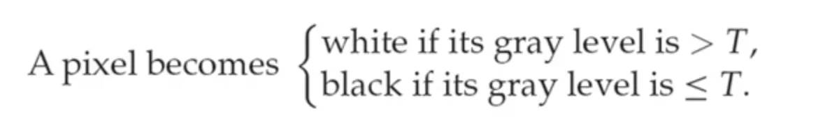
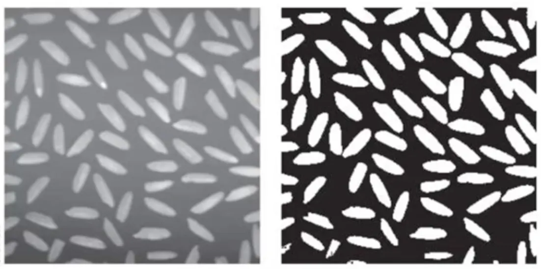
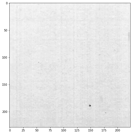
single thresholding 은 밝기값이 T 보다 큰 값은 흰색으로, 작은 값은 검은색으로 변경하여 binary image 로 만드는 알고리즘이다.
•
배경에서 영상을 분리하고 싶을 때
•
영상에서 육안으로는 잘 구분하지 못하는 외관을 보고 싶을 때
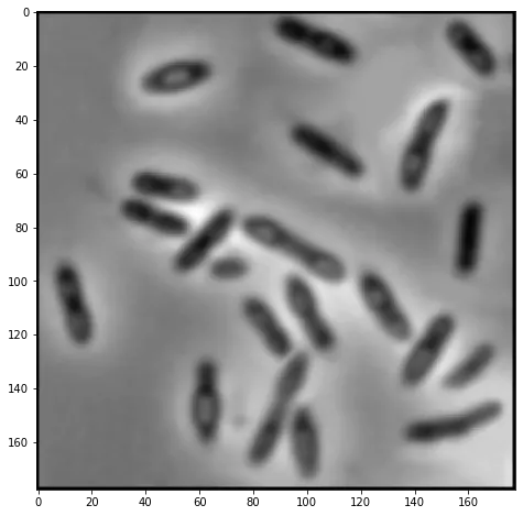
im = cv2.imread('bacteria.tif', cv2.IMREAD_GRAYSCALE)
plt.figure(111, figsize = [8,8])
plt.imshow(im, cmap='gray')
Python
복사
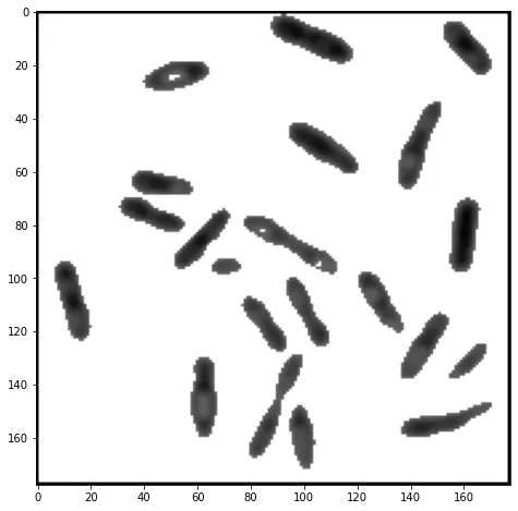
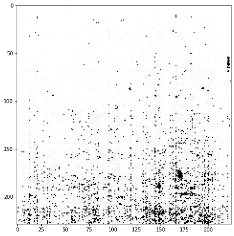
im[im > 100] = 255
plt.figure(112, figsize = [8,8])
plt.imshow(im, cmap='gray')
Python
복사
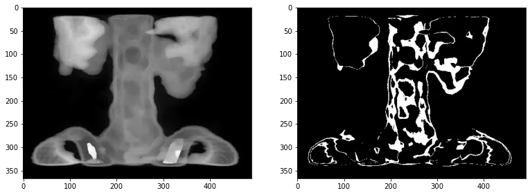
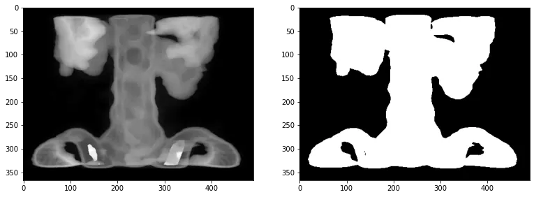
이중 문턱치 처리 (double thresholding)
im_spine = cv2.imread('spine.tif', cv2.IMREAD_GRAYSCALE)
plt.figure(114, figsize = [13,5])
plt.subplot(1,2,1)
plt.imshow(im_spine, cmap='gray')
cond = (im_spine > 115) & (im_spine < 125)
im_spine[cond] = 1
im_spine[~cond] = 0
plt.subplot(1,2,2)
plt.imshow(im_spine, cmap='gray')
Python
복사
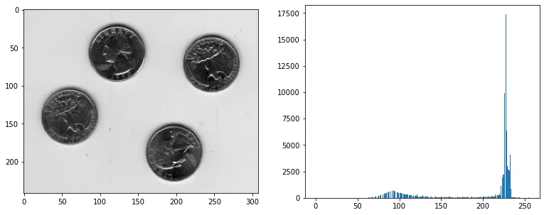
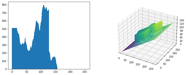
적절한 문턱치 설정
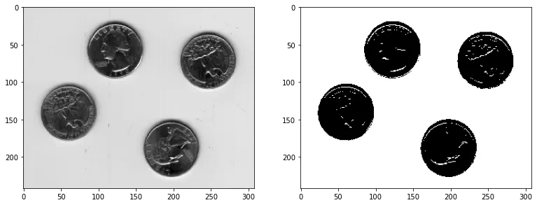
적절한 문턱치를 설정하기 위해 histogram 을 확인해보는 전략을 취할 수 있다.
im_conis = cv2.imread('coins.tif', cv2.IMREAD_GRAYSCALE)
plt.figure(115, figsize = [13,5])
plt.subplot(1,2,1)
plt.imshow(im_conis, cmap='gray')
x_range = [0, 255]
bins = 2**8 # 256
plt.subplot(1,2,2)
plt.hist(im_conis.flatten(), bins=bins, range=x_range)
Python
복사
•
위 histogram 을 보면, 약 150 정도의 문턱지를 설정하면 좋을 것이다.
•
하지만, 이렇게 설정된 문턱치는 이 영상에 대해서 제한적이다.
•
매번 다른 영상이 들어오더라도 적절한 문턱치를 찾을 수 있도록 진화해야 한다.
영상의 histogram 을 확률분포로 모사한 뒤, 이 분포를 적절히 나눌 수 있는 문턱치를 가져가는 전략을 통해 자동으로 문턱치를 설정할 수 있지 않을까?
Otsu 의 방법론
•
class 는 종류를 의미하는 것으로, 배경과 물체를 나누는 segmentaiton 을 한다고 한다면, 배경과 물체가 각각 1개의 class 를 의미한다고 생각할 수 있다.
•
inter-class variance 는 서로 다른 class 간의 차이를 의미한다.
Otsu 의 방법은, Inter-class variance 를 최대화하는 문턱치를 찾는 방법이다.
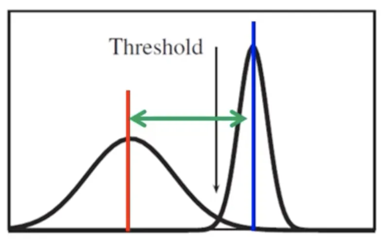
위 그림을 보자. red : class 1 의 평균, blue : class 2 의 평균일 때, 이 두 class 를 가장 잘 구분할 수 있는 문턱치를 설정한다는 말이 된다.
그렇다면 class 간의 차이를 의미하는 inter-class variance 를 Otsu 는 어떻게 정의했을까?

•
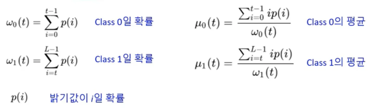
문턱치 가 변함에 따라서, t 보다 작은 영역에 속하는 확률분포가 class 0, t 보다 큰 영역에 속하는 확률분포가 class 1 에 속하는 확률분포 라고 생각해 보자.
•
각 확률 분포의 평균 을 구한다.
•
inter-class variance 는 각 확률 분포의 평균 차이의 제곱에 비례한다.
•
inter-class variance 는 각 클래스에 속할 확률의 곱에 비례한다.
수식을 바라보다 보니 문득 든 생각인데, 어차피 위 함수 를 최대가 되도록 만드는 t 를 찾는 것이기 때문에, 식을 이렇게 변경해도 될 것 같았다.
식을 이렇게 변경하게 되면, t 가 갈라놓은 두 확률분포에서, 각 클래스에 해당하는 확률값의 (확률분포의 아래 면적) 기하평균에 비례하고, 두 확률분포의 평균의 차이에 비례하는 어떤 함수를 가장 크게 만드는 t 를 찾는 문제라고 해석할 수 있게 된다.
def otsu(im):
t = 0
max_f = 0
for i in range(1, 256):
cond = im < i
x1 = im[cond]
x2 = im[~cond]
if len(x1) == 0:
continue
if len(x2) == 0:
continue
mu1 = x1.mean()
mu2 = x2.mean()
_, x1_counts = np.unique(x1, return_counts=True)
_, x2_counts = np.unique(x2, return_counts=True)
p1 = sum(x1_counts)
p2 = sum(x2_counts)
f = p1*p2*(mu1-mu2)**2
if max_f < f:
max_f = f
t = i
return t
def auto_thresholding(im, return_threshold=False):
im = im.copy()
t = otsu(im)
cond = (im > t)
im[cond] = 1
im[~cond] = 0
if return_threshold:
return im,t
else:
return im
plt.figure(116, figsize=[13,5])
plt.subplot(1,2,1)
plt.imshow(im_conis, cmap='gray')
ret, threshold = auto_thresholding(im_conis, return_threshold=True)
print("Thresholding with Otsu's method:", threshold)
plt.subplot(1,2,2)
plt.imshow(ret, cmap='gray')
Python
복사
물론 이렇게 구현해 쓰는 건 병렬처리와 연산 최적화가 되지 않기 때문에 느리고 성능도 별로다.
Thresholding with Otsu's method: 166
Plain Text
복사
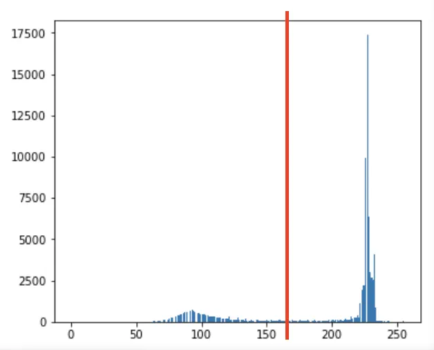
잘 - 찾았다!
plt.figure(117, figsize=[13,5])
plt.subplot(1,2,1)
im_spine = cv2.imread('spine.tif', cv2.IMREAD_GRAYSCALE)
plt.imshow(im_spine, cmap='gray')
ret, threshold = auto_thresholding(im_spine, return_threshold=True)
print("Thresholding with Otsu's method:", threshold)
plt.subplot(1,2,2)
plt.imshow(ret, cmap='gray')
Python
복사
Thresholding with Otsu's method: 64
Plain Text
복사
plt.figure(117, figsize=[13,5])
plt.subplot(1,2,1)
x_range = [0, 255]
bins = 2**8 # 256
plt.hist(im_spine.flatten(), bins=bins, range=x_range)
plt.subplot(1,2,2)
x_range = [0, 255]
bins = 2**8 # 256
plt.hist(im_spine[im_spine < threshold].flatten(), bins=bins, range=x_range, color='r')
plt.hist(im_spine[im_spine >= threshold].flatten(), bins=bins, range=x_range, color='b')
Python
복사

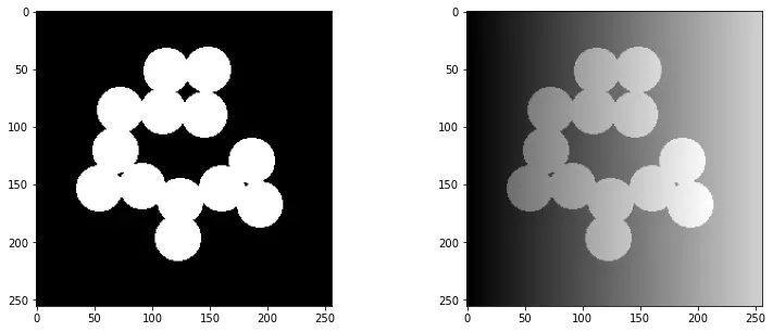
적응형 문턱치 처리
적응형 문턱치 처리가 필요한 상황을 임의로 생성해 보자.
from mpl_toolkits.mplot3d import axes3d
plt.figure(211, figsize=[13,5])
# ---
plt.subplot(1,2,1)
im_circles = cv2.imread('circles.tif', cv2.IMREAD_GRAYSCALE)
plt.imshow(im_circles, cmap='gray')
# ---
plt.subplot(1,2,2)
im_circles_noised = np.ones(im_circles.shape)
noise = np.linspace(0,im_circles.shape[-1]-1,im_circles.shape[-1])/2
mask = (im_circles == 0)
im_circles_noised[mask] = (im_circles_noised * noise)[mask]
noise = np.linspace(0,im_circles.shape[-1]-1,im_circles.shape[-1])/2+50
im_circles_noised[~mask] = (im_circles_noised * noise)[~mask]
im_circles_noised = im_circles_noised.astype(np.uint8)
plt.imshow(im_circles_noised, cmap='gray')
Python
복사
plt.figure(212, figsize=[13,5])
# ---
plt.subplot(1,2,1)
x_range = [0, 255]
bins = 2**8 # 256
plt.hist(im_circles_noised.flatten(), bins=bins, range=x_range)
# ---
ax = plt.subplot(1,2,2, projection='3d')
X = np.linspace(0, im_circles_noised.shape[1]-1, im_circles_noised.shape[1]).astype(np.uint8)
Y = np.linspace(0, im_circles_noised.shape[0]-1, im_circles_noised.shape[0]).astype(np.uint8)
X, Y = np.meshgrid(X, Y)
ax.plot_surface(X, Y, im_circles_noised, rstride=1, cstride=1,cmap="viridis")
Python
복사
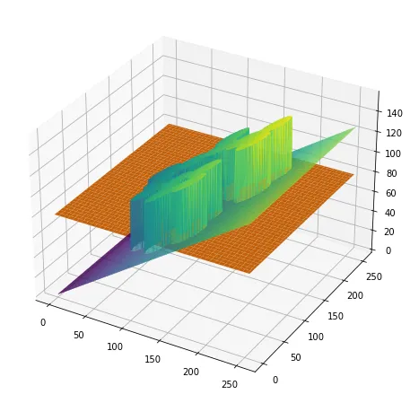
이런 상황에서, 단일 문턱치를 이용해 segmentation 하겠다는 것은 아래 코드와 같은 상황을 나타낸다.
plt.figure(212, figsize=[8,8])
ax = plt.subplot(1,1,1, projection='3d')
X = np.linspace(0, im_circles_noised.shape[1]-1, im_circles_noised.shape[1]).astype(np.uint8)
Y = np.linspace(0, im_circles_noised.shape[0]-1, im_circles_noised.shape[0]).astype(np.uint8)
X, Y = np.meshgrid(X, Y)
ax.plot_surface(X, Y, im_circles_noised, rstride=1, cstride=1,cmap="viridis")
t = 80
t_surface = np.ones(im_circles_noised.shape)*t
ax.plot_surface(X, Y, t_surface)
Python
복사
영상을 작은 부분으로 나누고, 각각에 대하여 문턱치 처리를 해 보는 방법을 생각해 볼 수 있다.
plt.figure(213, figsize=[8,8])
plt.subplot(1,2,1)
trial_1 = auto_thresholding(im_circles_noised)
plt.imshow(trial_1, cmap='gray')
plt.subplot(1,2,2)
trial_2_1 = auto_thresholding(im_circles_noised[:,:50])
trial_2_2 = auto_thresholding(im_circles_noised[:,50:100])
trial_2_3 = auto_thresholding(im_circles_noised[:,100:150])
trial_2_4 = auto_thresholding(im_circles_noised[:,150:256])
plt.imshow(np.concatenate([trial_2_1, trial_2_2, trial_2_3, trial_2_4], axis=1), cmap='gray')
Python
복사
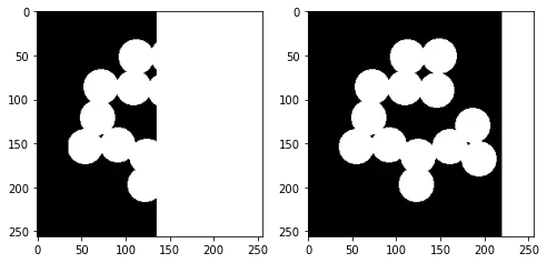
좌측은 단순히 Otsu 의 방법을 사용했을 경우이고
우측은 네 영역으로 분할한 뒤 각각에 Otsu 의 방법을 적용한 경우이다.
이런 방법들 외에도, 정말 다양한 아이디어를 낼 수 있을 것이라고 짐작할 수 있다. 이 강의에서는 segmentation 에 대해서 여기까지만 다룬다. 앞으로 나올 edge detection 에서도 너무 깊이 들어가지 않고 가볍게 다룬다.
에지 검출 (edge detection)
에지 (edge) 는 주어진 문턱치를 초과하는 픽셀값들의 국부적인 불연속을 의미한다.
경사 에지 (ramp edge) 는 밝기값이 서시히 변하는 에지를 의미한다.
계단 에지 (step edge) 는 밝기값이 급격히 변하는 에지를 의미한다.
프로파일 (profile) 과 미분 (derivative)
프로파일 (profile) 은 어떠한 변화를 의미한다.
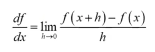
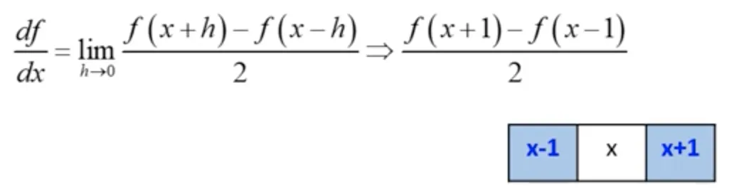
어떤 미분가능한 함수에서 도함수는 아래와 같이 표현한다.
그런데 영상에서 가장 작은 변화의 단위는 1 이다.
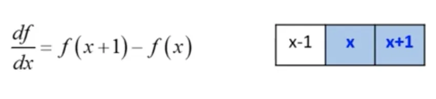
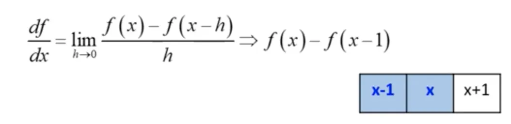
이것을 조금만 더 확장해서 생각해서, 최소단위가 2라고 생각해도 무리가 없다.
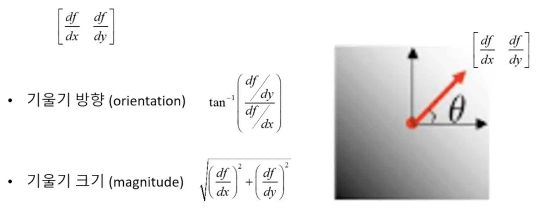
기울기 (gradient) 와 편미분 (partial derivative)
기울기 (gradient) 는 함수 f(x,y) 에 대해서 밝기값이 증가하는 방향의 벡터이다.
사실 꼭 증가하는 방향으로 정의할 필요는 없는 것 아닐까. 하지만 이렇게 약속함으로써, 오른쪽과 윗쪽은 항상 +, 왼쪽과 아랫쪽은 항상 - 모양의 필터들만 찾을 수 있게 되었다. 그리고 오른쪽과 윗쪽의 f(x+h) 에서 왼쪽과 아랫쪽의 f(x-h) 를 빼 주는 형태가 되었다. 이렇게 된다면 연산의 결과가 반드시 밝기값이 증가하는 방향의 벡터만 나오게 된다. 이렇게 무엇인가를 관례적으로 약속해두면 생각이 상당히 간단해지곤 한다.
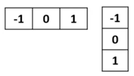
에지 검출 필터
을 도함수로 여기고 필터로 만들면 된다.
그런데 여기서 검출하려는 방향의 반대 방향으로 복사-붙여넣기 한 형태의 필터는 smoothing 의 역할을 한다. 앞서 영역 단위 영상처리 연산과 필터링 과 영상의 열화와 복원 에서 배웠듯, 커널 (필터) 의 사이즈가 커지면 국소적인 노이즈에 강인해지지만 디테일이 사라지는 등의 문제가 있었던 것을 기억하자.
영역 단위 영상처리 연산과 필터링 과 영상의 열화와 복원 에서 배웠듯, 커널 (필터) 의 사이즈가 커지면 국소적인 노이즈에 강인해지지만 디테일이 사라지는 등의 문제가 있었던 것을 기억하자.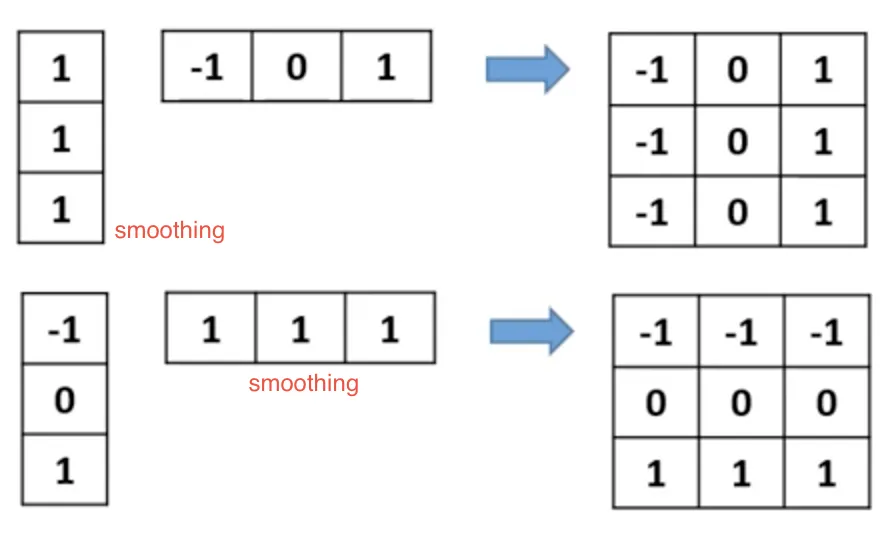
이렇게 생긴 filter 들을 Prewitt filter 이라고 한다.

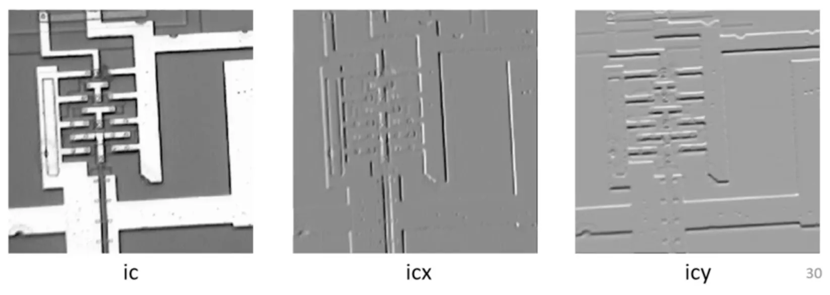
좌측 : 원본, 중앙 : x 방향 에지 검출기, 우측 : y 방향 에지 검출기

x 방향 에지 검출기가 만든 결과를 가까이서 들여다 보자. 위 이미지 조각처럼 경계에서는 "픽셀값이 밝아지는 방향" 이 다르기 때문에, 에지 검출기로부터 나타나는 밝기값이 완전히 반대이곤 하다. (하양, 검정).
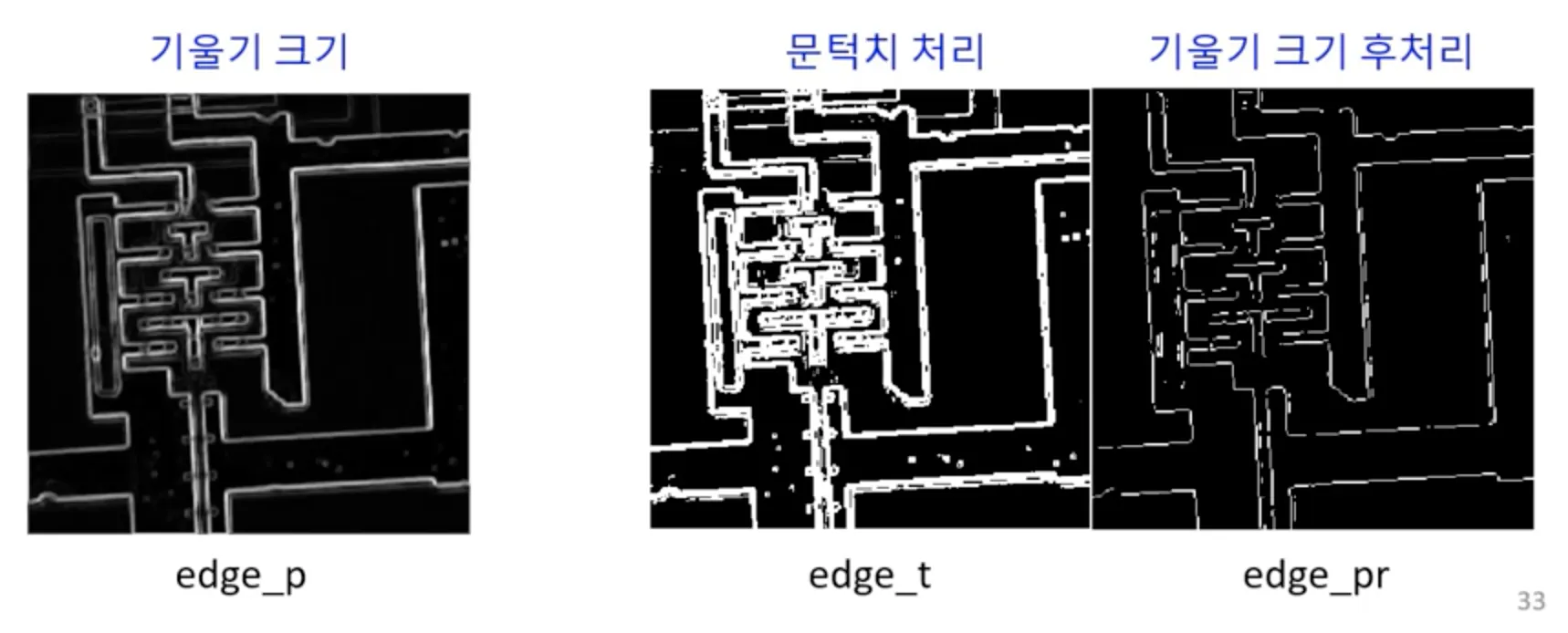
기울기의 크기를 구하는 연산을 거치면 edge_p 가 된다. 그리고 threshold 를 이용해서 일정한 기준으로 에지인 것과 아닌 것을 구분해 주면 edge_t 의 결과를 얻을 수 있다.
추가 자료